I. What is a point cloud
Point clouds are a mathematical sets of 3D points with x,y,z coordinates and with or without attribute(s). The attribute of a point cloud can be its R,G,B color indication, its class or the type of object it belongs to (ground, low vegetation, table, etc) or any other properties such as intensity, time of capture, etc. Point clouds are used to describe objects’ properties such as shape, texture, color in 3D space.
Their application span accross many areas including building and construction, road engineering, vegetation and infrastructure monitoring, automotive.
Below is an example of a point cloud scene from an urban area viewed in Cloud Compare: an indispensable open source tool for viewing and processing point cloud. Each color in the scene represent a different type of object as classified by KPConv, the kernel based point convolution neural network we will talk about soon.

II. KPCONV’s architecture
The architectural design of KPConv follows the well known encoder-decoder architecture used in 2D image segmentation task: each block of the encoder network is inspired by ResNet’s blotteneck residual block while the convolution operation is applied to the set of points in the Euclidian space; the convolution in KPConv is referred to as kernel point convolution.
We will follow a top-down approach to describe the structure of the network.
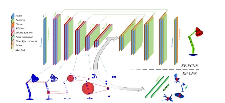
KP-FCNN stands for Kernel Point Fully Convolutional Neural Network and used for segmentation tasks (including scene segmentation, part segmentation) while KP-CNN (Kernel Point Convolutional Neural Network) is used for part classification.
Each encoder layer is a residual block comprised of normalization, kernel point convolution and activation operations. Inputs to the first layers are points subsampled at a grid size of \(dl_0\); each point contains its supports coordinates in Euclidian space x,y,z and its intensity and/or color features. In addition, a constant 1 is added as feature to each point to avoid dealing with empty space in case the point cloud is without any feature. In the following layers, the number of points is reduced by a grid size \(dl_i = 2^i \cdot dl_0\) where i is the layer index starting from 0.
Parallelly, the depth of the network is increased by \(64*2^i\) with the kernel size. This is illustrated with the red sphere growing proportionally with the decrease of the number of points in blue. The feature at each new location is pooled with a strided kernel point convolution.
The decoder layer is made of nearest up sampling plus concatenation with the corresponding encoder’s layer followed by a unary convolution. The kernel point convolution is applied directly to the points without any transformations as is the case in projections-based network for example. It owes its mathematical expression to the initial work on point convolutional networks namely PointNet [2].
Given \(x_i\) , \(f_i\) respectively the set of points coordinates and features, the kernel point convolution (KPConv) \(F\) by a kernel \(g\) is defined by \[F(x)=∑_{x_i} g(x_i-x) f_i\]
where \(g(x_i-x)\) is the kernel function defined in the spherical neighborhood of radius \(r≥x_i-x\).
KPConv singularities lie in the kernel function centered in x. We want the kernel to apply different weights in the neighborhood. Given K kernel points, we want the kernel for each neighbor point in the ball to be proportional to the distance from the point to the kernel points. More specifically \[g(y_i )=∑_{k<K} h(y_i,k) W_k \] where \(y_i\) is the neighbor point, k represents the kernel point and \(W_k\) its weights.
h is the correlation function defined by \[h(y_i,k)=max(0,1-\frac {||y_i-k|| } {σ}) \] which is higher if the neighbor point is close to the kernel point and lower when it is not but can’t be negative.
Following the definition of the kernel function, one understands the importance of the disposition of the kernel points: the disposition of the points should be representative of the spherical local neighborhood. We can define this as follows: how can we choose K points so that these points are as far as possible from each other in the sphere but also centered around the center. This problem is equivalent to solving a spherical Voronoi diagram of K points by solving the optimization problem with a constraint defined by the repulsive energy of each point vis-a-vis of other neighbors’ points added to its attractive energy vis-a-vis of the center point. This kernel disposition is used in the rigid version of KPConv.
It is also possible to learn the optimal kernel dispositions by learning the shift to be applied to the rigid kernel disposition as it is the case in the 2D deformable convolutions. And to avoid having dispersed kernel points, a new loss is formulated to penalize grouping of points and influence area overlapping of the shifted points. This new disposition of the kernel points is what makes deformable KPConv which can be used in the network in the same way as the rigid version.
The network can be trained to minimize cross-entropy loss with momentum gradient Descent algorithm.
The influence area of kernel point convolution is defined by its radius which is usually \(r_j= 2.5*σ_j\) for rigid KPConv and \(r_j=ρ*dl_j\) where \(σ_j=dl_j*ϵ\) and \(ϵ=1,K=15,ρ=5.0\).
\(σ_j, K ,ρ\) are respectively the kernel point influence distance, the total numbers of kernel points and the deformable kernel influence.
III. Processing and loading point cloud data for KPConv
Points clouds scenes can be very large and have different density across regions, that’s why it is important to first subsample input clouds using a grid subsampling method where the barycenter of the grid is the only point picked to replace other points in the grid. The subsampling rate \(dl_0\) or the size of the cubic grid is a tunable parameter depending on the type of data; set it too high and the algorithm will fail to learn local and close features of points, set it too low and the algorithm will fail in learning general properties such as shapes, texture of big scenes. This is by far, the first parameter to be tuned to fit your use case.
Since it is impractical to load all points in all scenes at once due to their large numbers, we use spheres to load data. The larger the sphere the more context we provide to the network and the higher is the memory use. The radius of such sphere is also a parameter to be tuned but the rule of thumb is to start with a value of \(R=50*dl_0\) and reduces this if required. We can even go farther and make an analogy with 2D computer vision tasks: the input spheres are like the region of the big dataset scene where we zoom in at a time just like an image is like the region of the whole dataset (see the image dataset as a concatenation of all the images present in it) we look at a time.
For example, it is very common to have a high number of ground points, hence the importance of having a larger input sphere as this also means the network can see and learn contexts of different object types at once.
Now arrises the question of how to pick those spheres so that all points are given the chance to be seen by the network. One way is to randomly pick spheres centers from the big scene (concatenated scenes) until a given number of spheres is reached. The weakness of such an approach lies in its sensibility to varying densities: areas with more points such as vegetations and grounds have a higher probability of being picked. If used for training, this can harm the learning and create less robust predictions, and such an approach is definitely not advised for testing as all the points won’t be seen by the network.
Instead, one can spatially and regularly pick spheres centers so that each point is at least seen by the network and picked spheres come from different regions. This can be done by keeping track of the points in picked spheres by updating their Tukey weights or simply potentials of being picked every time we select a sphere center. Next time, we will simply pick from the region where the potential is the lowest.
\(Tukey(x) = 1-\frac{(||x_c-x||)} {d_{Tuk}^2} ^2\) if \(||x_c-x||≥d_{Tuk}\) else \(Tukey(d)\)
where \(d_{Tuk}=\frac {R}{3}\) defines the reach of the Tukey weights inside the spheres. This definition of Tukey potentials will give lower weights to points close to the surface of a sphere of radius \(\frac {R}{3}\) and higher weights to those close to the center. Initially, the potentials are initialized with small random numbers and updated after every picking. The next sphere center is picked where the potential value is the minimum. We can continue picking the spheres until all points are picked, and during predictions in production or test, we can define the minimum number of times a point is to be seen by the network and average the predictions: this is referred to as voting scheme in KPConv paper[1].
For geometric consistency reasons, it is advantageous to have variable batch size. For example, while many point clouds are needed to describe ground or flat surfaces, fewer are needed to represent a traffic object. KPConv uses stacked batches where all input points are stacked on their first dimension (number of points).
A calibration method is used to make sure the average input spheres in the batch is equal to a predefined value of the given batch size. Basically, we use a P controller to find the maximum number of points to be processed in a batch.
Because some regions are dense and having too many neighbors can cause an OOM error, we apply a low pass filter to keep only 80 to 90% of neighborhoods’ points. This does not affect learning as points in dense regions are the ones affected by the filter and are usually redundant.
As data augmentation, we can use vertical rotation where the input sphere is rotated vertically, and anisotropic scaling consists of applying non-uniform scale to the points along x axis.
Below is an example of a point cloud classified using KP-FCNN.

References
- Thomas, Hugues, et al. “Kpconv: Flexible and deformable convolution for point clouds.” Proceedings of the IEEE/CVF international conference on computer vision. 2019.
- Qi, Charles R., et al. “Pointnet: Deep learning on point sets for 3d classification and segmentation.” Proceedings of the IEEE conference on computer vision and pattern recognition. 2017.